Enhance your holiday snaps with histogram equalisation
The problem --
Manual fix --
Histogram equalisation --
Source and parameters
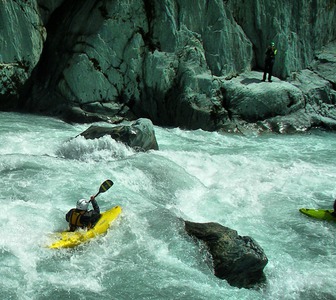
The bright sun of New Zealand
On a recent vacation, my camera reached the
lower limit of its range of exposure times. Apparently the relative proximity
of New Zealand to the equator compared to Europe and the great weather were too
much. What is more, the regions in the shadow turned out uniformly dark
compared to those in the sun. The upshot was that the photos were not unusable
or ugly, but lacked contrast in different image regions while the contrast
between sunny and shadowy regions was stark. This problem was especially
noticeable in photos on the river on bright days, where the foam and waves
cause bright reflections.
Manual correction
The most obvious way to enhance such images — that are partly
overexposed and partly underexposed — is to postprocess them manually
with an image manipuilation program such as GIMP .
Just adjusting brightness and contrast may be sufficient for photos that are
either underexposed or overexposed, but for pictures with regions of both, it
will not do. For those, you need a more general transformation of pixel's
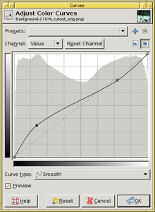
brightness, which is provided by GIMP's curves tool (Colors -> Curves or Tools
-> Color Tools -> Curves in the context menu). It allows enhancing (i.e.
stretching) those intervals of brightness that are overused at the expense of
compressing those that are little used. This results in better contrast for
both bright and dark region (with the little-used intermediate brightnesses
compressed).
.
Just adjusting brightness and contrast may be sufficient for photos that are
either underexposed or overexposed, but for pictures with regions of both, it
will not do. For those, you need a more general transformation of pixel's
brightness, which is provided by GIMP's curves tool (Colors -> Curves or Tools
-> Color Tools -> Curves in the context menu). It allows enhancing (i.e.
stretching) those intervals of brightness that are overused at the expense of
compressing those that are little used. This results in better contrast for
both bright and dark region (with the little-used intermediate brightnesses
compressed).
The images above show an example. Here the dark regions are more problematic
than the bright ones — the crevice on the left is blacked out and the
person standing on the right in the background is almost invisible. Increasing
the slope of the brightness curve where the histogram has peaks increases
contrast there. (Note that the histogram is logarithmic, so the peaks are more
pronounced than they may seem.) As a result, the person standing on the rock
is visible in the processed image (right), and the crevice and the rock in the
foreground show more structure. The foamy regions of the water have gained a
little contrast, too.
Histogram equalisation
To my discredit, it was only after manually correcting hundreds of photos that
I remembered the more-or-less automatic method for doing such corrections. (In
fact, my father did most of the manual corrections. He is retired and hates
bad photos.) To see the principle, let us again go over what we have done when
correcting the brightness manually. We applied a transformation function to
the brightness of each pixel that had a large slope where many pixels had a
similar brightness and a small slope where few pixels were. That stretched the
regions of the brightness histgram with a high pixel density and compressed
those with a low density. Simply put, we have reduced the variation of the
histogram, made it flatter.
The method we have applied manually is well-known in the image processing
literature as "histogram
equalisation " (HE). In fact the original form of this method may be too
extreme, as it makes the histogram completely flat. (Strictly speaking, this
is only true when the histogram is averaged out. The method is deterministic
and cannot increase the total number of different brightness values, so some
values do not occur at all in the result image.) Two improvements have been
invented over the years:
" (HE). In fact the original form of this method may be too
extreme, as it makes the histogram completely flat. (Strictly speaking, this
is only true when the histogram is averaged out. The method is deterministic
and cannot increase the total number of different brightness values, so some
values do not occur at all in the result image.) Two improvements have been
invented over the years:
- Contrast limiting — transform the image as for histogram
equalisation, but do not go the whole way. The slope of the transformation
function is limited so that the contrast enhancement does not become too
extreme. This is known as contrast-limited HE or CLHE.
- Adaptiveness — each pixel is not transformed in the same way, but
depending on the histogram of a neighbourhood region. Different regions of
the image are then enhanced independently of each other, with better results.
This is called
AHE or, when
combined with contrast limiting, CLAHE.
So what does the result of histogram equalisation look like for our test image?
Here it is:

This looks less enhanced than the manual result above. The cliff face is
darker, and the person less visible. In fact, displaying a histogram with GIMP
shows that I have been overdoing it a bit with the manual correction. The
brightened cliff produces a different peak in the histogram from before, and
the peak on the right from the water partly remains. (You can see the
histogram of the original image in the curves dialog above.) The histogram of
the HE-processed image is indeed completely flat on average. The darker parts
of the water have been darkened still more, increasing contrast there and
erasing the corresponding peak in the histogram. The cliff has been brightened
enough to flatten the left histogram peak, but not enough to make the standing
person or the interior of the crevice clearly visible.
This is a bit disappointing for a state-of-the-art image processing method. So
can it be fixed? As mentioned above, a variant called CLAHE allows enhancing
different regions of the image independently. We apply it to the image,
choosing 8 by 8 tiles and an amplification limit of 1.7 (see below
about these parameters):

Now the inside of the crevice is better visible, and so is the standing person,
if only slightly (click on the images to see larger versions). But the
structure of the cliff face is much enhanced. This is a consequence of the
adaptivity of this method, which allows treating that image region
independently. The water turbulences also have more contrast than in any of
the previous result images.
But there are a few drawbacks too: The PFD (life jacket) of the paddler is
darker than in the previous attempts, and the darker regions of the water look
a bit grey (this was also true in the previous results). This is because these
pixels are among relatively few dark ones of their neighbourhood region, and
are therefore darkened more still. The human eye perceives darker pixels as
less colourful, which makes the result less appealing. But one can apply
histogram equalisation to any quantity of a pixel, not just the brightness. By
transforming the colour saturation instead, one can intensify the colours. (It
seem I invented this application, at least I have not read this anywhere.)
Contrast limiting has to be used, or the colours will turn out psychedelic.
Adaptiveness helps to concentrate the enhancement on the most colourful spots,
so I use 8 by 8 tiles again, and a magnification limit of 1.3. The result is:
The colours are more intense; besides the paddler the water is also greener.
Unfortunately the rock face also has a greenish tinge, but that is something
for which my camera is mostly to blame.
So what have we learned? Histogram equalisation is a powerful method that can
help a lot in improving the quality of images. Its different variants and
parameter values have their individual advantages and disadvantages, both
compared with each other and compared to a global manual contrast enhancement.
There is no fully automatic method that produces what you consider perfection.
But experimenting with them a little can help with degraded images.
Source code and parametrisation
I have written a C program performing histogram equalisation that is pretty
generic. The source code is here. It is designed for
versatility rather than performance or comfort and can process only
PNM images (but see below for a wrapper
script). It can process both greyscale and colour images with up to 16 bits
depth.
The program can take a number of parameters, most of which relate to the
histogram equalisation method to apply:
- To perform contrast limiting, the limit has to be specified. pnmclahe
takes the option -l followed by a normalised limit value that can be
thought of as the maximum amplification of the transformation anywhere in the
range of brightness values. It may be fractional. The default is 3. This
parameter is often called the "clip limit", because of how it is used by the
method.
- Adaptive histogram equalisation requires specifying the size of the
neighbourhood region used to transform each pixel. To make the method
computationally feasible, the image is divided up into tiles of (almost)
equal size between which the transformation is interpolated (see
Wikipedia).
Therefore this parameter takes the form of giving the number of tiles.
pnmclahe accepts the option -t with an argument like 5x4, meaning
5 tile columns and 4 tile rows. The default is 1x1, a global
non-adaptive transform.
The third command line option is -s which enables transforming the colour
saturation rather than the brightness. pnmclahe defines the brightness of
a colour pixel as the largest colour component and transforms the other
components proportionally. The colour saturation is defined as the difference
between the largest and smalles colour components, and its transformation is
linear so that the interval below the smalles and above the largest colour
component keep the same ratio.
Running pnmclahe without arguments or with the -h option makes it
output a usage message.
To apply pnmclahe to images in any format, it is advantageous to write a
wrapper shell script which also contains appropriate
ImageMagick convert commands.
This shell script is an example. Besides format conversion, it
also saves the original image in a subdirectory and uses that backup as a
source image on second and later runs. It also copies
EXIF metainformation from the original
image to the end result.
TOS / Impressum