| ↑↑↑ Home | ↑↑ Science | ↑ Papers |
The Mann-Whitney-Wilcoxon (MWW) test is a statistical two-sample test, that is, a test which compares two sets of numbers. It comes in two forms. The first tests the null hypothesis that the two samples belong to the same distribution. This is the so-called two-tailed test. The second form tests the null hypothesis that either both samples have the same distribution or that the first sample is larger in a statistically significant way. If the null hypothesis can be rejected in this so-called one-tailed test, it can be concluded that the second sample is in fact larger. A strength of the MWW test in general is that it is distribution-free, i. e. it implies no assumptions about the actual distribution of the two samples. It is frequently used in the social and life sciences.
Here, only the one-tailed test will be considered. Besides, in the following discussion it will be assumed that all elements of the combined two samples are different. The formulae which will be derived will follow Mann and Whitney's formulation of the test; the formulation of Wilcoxon is slightly different.
The MWW test is a permutation test. It based on the idea that if the two samples have the same distribution, any quantity which you can compute from them will be invariant under permutations of values between, rather than just within the two samples. The quantity which is central to the MWW test in Mann and Whitney's formulation is called Mann-Whitney U:
Clearly, U cannot exceed |S1|*|S2| and will reach that limit only when all elements of S1 are larger than those of S2. The smaller U, the higher the significance with which S1 can be pronounced smaller than S2. (The one-tailed test is sometimes formulated the other way round, with the null hypothesis being that both samples have the same distribution or S1 is smaller than S2. Then a sufficiently large U indicates that S1 is larger than S2.)
The combinatorial problem which we will use to compare programming languages is
to compute the significance of this test exactly. There is an approximation
which is acceptable for all but the smallest sample sizes (see Wikipedia ), but here we will perform the exact computation. To do
so, one has to compute the
probability that two samples drawn from the same distribution result in the
same or a smaller U. The number of possibilities of dividing
|S1|+|S2| values into two samples of size |S1|
and |S2| is given by the binomial coefficient
), but here we will perform the exact computation. To do
so, one has to compute the
probability that two samples drawn from the same distribution result in the
same or a smaller U. The number of possibilities of dividing
|S1|+|S2| values into two samples of size |S1|
and |S2| is given by the binomial coefficient ![]() . It remains to count the different choices for
S1 (and the corresponding S2) which result in a
Mann-Whitney U less than or equal to the given U (which is obtained by applying the formula for U to the data under consideration).
. It remains to count the different choices for
S1 (and the corresponding S2) which result in a
Mann-Whitney U less than or equal to the given U (which is obtained by applying the formula for U to the data under consideration).
As explained briefly in the previous section, we want to compute the number of divisions of a set of numbers into two samples of given sizes so that a given maximal Mann-Whitney U is not exceeded. In this section we will choose a suitable parametrisation and develop the algorithm we will use in the implementations below.
Considering the nature of the MWW test, the actual values drawn from the hypothetical distribution do not matter; U depends only on how they compare. We will assume them all to be different, and can without loss of generality think of them as the naturals from 1 to |S1|+|S2|. To simplify our notation, we will make some abbreviations. We will define n:=|S1|+|S2|, m:=|S1| and denote the given Mann-Whitey U with a small u.
Our task is now to consider all choices for S1 from the set {1,..,n} so that |S1|=m and count those for which U(S1, S2={1,..,n}\S1)<=u. The result will be called l(n,m,u). The straightforward way of computing l would be to loop over all possible sets S1 and compute U for each of them. This is obviously the simplest way of doing it and will be improved upon. But let us first develop a parametrisation which allows us to consider each S1 exactly once. The parameters we choose are the numbers of values belonging to S2 between neighbouring elements of S1 when both samples are sorted together and written down in order. We denote these "gaps" in S1 by di. If there is no element of S2 between successive values of S1, then the corresponding di=0. The following example demonstrates the concept. The numbers called s1(..) are the elements of S1, the s2(..) are in S2, and in this example s2(1) is the smallest element of the complete sample.
To select a specific S1, we will work our way up from the smallest values, first choosing d0 (the number of values starting from the smallest which belong to S2; d0 is 0 if the smallest value belongs to S1). Then we compute the effect the following value, which is an element of S1, will have on the total U. It is clear that this smallest element of S1 will contribute exactly d0 to U, because it exceeds the d0 smallest elements of S2 but no others. Wouldn't it be nice if we could recurse and continue analogously with d1? In fact this is possible:
In order to treat all di equally, we have to compute at each stage not only the contribution of the current element of S1 to U, but also the amount by which the contribution of all larger elements of S1 is made larger by the preceding elements of S2. We do this by regarding the given u as a budget from which we subtract these contributions. How much do we have to subtract? As stated above, the contribution of the first element of S1 is d0. The contribution of each of the other m-1 elements becomes larger by d0 because of these first elements of S2: They are smaller than all higher-up elements of S1. So in total we have to subtract m*d0 from our u budget. If it becomes negative, we know that the originally given U has already been exceeded, so we can abort the recursion early.
Our algorithm can be written as the following recursion formula:
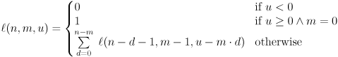
This is what we will implement.
In choosing the test cases for the benchmark comparison, I was influenced by the particular problem for which I had considered using the MWW test. In that application, the sizes of both samples are equal, so I chose them to be equal in the test cases as well. As a consequence, n=2*m in all cases. All the programs take m and u as their arguments, while n is omitted. The values chosen for m were a compromise: large enough for the runtime of the faster programming languages to be measurable but small enough that running the slower implementations was still feasible. The following table shows the three test cases and the computation results:
| m | u | l(2m,m,u) | Dead ends | Recursions | |
| 14 | 100 | 21863028 | 40116600 | 2577355 | 37694806 |
| 16 | 100 | 91520024 | 601080390 | 22710753 | 153132717 |
| 22 | 70 | 21266626 | 2104098963720 | 30545833 | 56321707 |
The fourth column shows the number of choices of m out of 2m items, the total possibilities of choosing the two samples. This is given only for illustration, as our algorithm does without searching through all of them. The "dead ends" are the number of times the selection of the di has to backtrack without finding a solution, that is the number of times the first branch in the recursion formula above applies. The last column shows the total number of calls to the function l(n,m,u) if the algorithm is implemented recursively, or equivalently the total number of stack push and pop operations for an iterative implementation (see below).
The columns which are relevant for the computational complexity of the task are the first, the third, and the last two. The first column, m, determines the maximum depth of the recursion. The third, the end result, gives the number of increments to the variable containing the result. The last two columns (especially the last) determine the amount of recursion (or stack management) necessary to obtain the result. So our second test case is a variant of the first which is more computationally expensive in all respects. The third test case, however, has approximately the same result as the first, but a larger maximum recursion depth, and requires a more complex search of the tree of choices for the di to arrive at the result.
The purpose of this investigation was to compare programming languages and to some extent their variants and implementations. The programming languages considered primarily were C, Perl, Haskell and Java. C (next to Fortran) is the traditional choice for scientific computing, and still often regarded as delivering the best performance. Perl is a script language one does not associate with serious number-crunching, but which allows quick coding of small utilities for day-to-day tasks. Haskell is a pure functional programming language which is close to mathematics in its notation. Java is a just-in-time compiled language which has been reported as now providing performance on a par with C. Two other languages were tested more or less systematically, mostly because they support arbitrarily large integers natively. They were Ruby, a multi-paradigm language that has evolved from Perl and others, and bc, a calculator available on all UNIX systems.
Besides comparing programming languages, we will take a look at parallel processing. In the forseeable future, processors will not primarily become more powerful through increases in clock frequency, but by having an increasing number of processing cores. This part of the investigation will center on the language C and compare different ways of parallelising the task.
Lastly, a comparison between different variants of the same languages was performed. Different compilers were tested for C and Java. Because the application of the MWW test I originally aimed at would have required integers wider than 64 bits, and because some languages natively support arbitrarily large integers, 64-bit implementations and large-integer implementations are compared separately. In most cases, both a recursive function implementation and an iterative (loop) implementation was tested. For the latter, the tree search of the values for the di was implemented using a manually allocated stack. Two large-integer packages available for Perl were also compared.
All tests were carried out on a dual-core Intel Core2 Duo 6600 processor running at 2.4 GHz, with 1 GB of RAM. The operating system used was Ubuntu Linux 6.06 x86_64 with a 2.6.23.8 kernel. For the duration of the tests, the computer was otherwise idle. The versions of the compilers or interpreters and supplementary packages used are listed in the table below.
| C | Gnu gcc | 4.0.3 |
| C | Intel icc | 9.1 |
| C | GMP library | 4.1.4 (libgmp.so.3.3.3) |
| Perl | Interpreter | 5.8.7 |
| Perl | bigint | 0.07 |
| Perl | Math::BigInt::GMP | 1.24 |
| Java | Gnu gcj/gij | 4.1.0 |
| Java | Sun JDK/JRE | 1.5.0_06 |
| Haskell | GHC | 6.8.2 |
| Ruby | Interpreter | 1.8.7 |
| bc | Gnu | 1.06 |
Before we start looking at runtimes, here is a very approximate comparison of the time it took to code the algorithm in each language. Some people maintain that this is even more important than runtimes, as programmer time is much more expensive than computation time. Though coding time has to be considered, I do not think this is true in most cases. Often a computation is part of an iteration of trying to solve a larger problem, with successive changes depending on the previous round's result. Then a slow computation can waste a lot of human time, and putting some effort into reducing runtimes will pay off. In my experience, the case where a numerical program is coded to be run only once or twice is extremely rare. In those cases, it certainly makes sense to choose the programming language which is quickest to code.
| Language | Development time |
| C | ≈ 1 day |
| Perl | Hours |
| Java | ≈ 1 day |
| Haskell | Hours |
| Parallel C | Days |
This table has to be taken with a pinch of salt. It reflects not just properties of the languages, but also which programming languages I know well (C and Perl), and which I do not (Haskell and Java). That said, Haskell looks an especially interesting option for quick coding, in particular for a mathematical problem such as the one we consider here. Despite having very little experience at it, I managed to write the program rather quickly. In addition, it left me with the feeling that the other implementations benefited from my previously working with Haskell, as its spartan, mathematical notation helped to concentrate on the algorithm. This advantage may not apply to problems less purely mathematical than this one, or to programmers less theoretically interested than me.
That Perl allows quick coding is probably no surprise. It is known as a language for quickly writing small utilities, and its weak typing, intelligible error messages and DWIM (Do What I Mean) principle all help to keep down development time. Java might be slightly faster to code than C for someone who knows it better than I do. Lastly, the parallel C implementations were most time-consuming. This may be due to that fact that I am no expert at parallel programming and that there were some unexpected effects, which are discussed below.
Ruby and bc were omitted from the development time table, as I wrote these implementations last. Due to having coded the algorithm several times before, the last implementations mostly amounted to copying. Both languages would probably rank with Perl if the program had been coded from scratch in one of them.
Runtimes were determined using the time command. The time used for the comparison was the wallclock ("real") time, not CPU time: If a program has to perform some IO for some unknown reason, that will slow it down and should be counted towards its total. The mean of at least three runs was taken unless the runtime was larger than a quarter of an hour. If the first run showed a significantly larger run time than the following runs, that was ascribed to the program, interpreter or auxiliary files being loaded into memory, and the run was discarded. For the compiled languages, the compile time was not included in the benchmark.
The following table gives the runtimes for the 64-bit implementation. The first column gives the language and the compiler/interpreter, the second shows whether the implementation was recursive or iterative. The following columns show the programs' runtimes for the three selected sets of arguments. The rows starting "Java Gnu compiled" contain the results for Java code compiled to native machine code with gcj (not bytecode interpreted). While compiling Java code to native machine code precludes distributing byte code compatible across systems, this is primarily of interest for preserving trade secrets (which distributing the source code would not), not usually a concern in a research environment.
| Language | Implementation | 14/100 | 16/100 | 22/70 |
| C gcc -O3 | recursive | 0.36 s | 1.1 s | 0.36 s |
| C gcc -O3 | iterative | 0.27 s | 0.94 s | 0.15 s |
| C icc -O3 | recursive | 0.43 s | 1.47 s | 0.38 s |
| C icc -O3 | iterative | 0.18 s | 0.66 s | 0.11 s |
| Perl | recursive | 46 s | 3 min 6 s | 1 min 4 s |
| Perl | iterative | 29 s | 1 min 44 s | 19 s |
| Java Gnu | recursive | 19.7 s | 1 min 20 s | 28.8 s |
| Java Gnu | iterative | 3.1 s | 10.5 s | 1.9 s |
| Java Gnu compiled -O3 | recursive | 0.41 s | 1.46 s | 0.53 s |
| Java Gnu compiled -O3 | iterative | 0.29 s | 0.92 s | 0.21 s |
| Java Sun | recursive | 0.35 s | 1.23 s | 0.46 s |
| Java Sun | iterative | 0.39 s | 1.1 s | 0.28 s |
| Java Gnu gcj / Sun JRE | iterative | 0.39 s | 1.1 s | 0.28 s |
| Java Sun JDK / Gnu gij | iterative | 3.1 s | 11 s | 1.9 s |
The first four rows show that gcc is better or worse than the Intel compiler, depending on the program: gcc is better with the function-recursive code, while icc is better with the iterative implementation. As expected, Perl is much slower than C (about by a factor of 100). If the program is not to be run too often and with too large parameters, its ease of coding and modification (see below) might still make it an option, though.
Java lives up to its new reputation as a real alternative to C and other compiled languages, but not with the Gnu bytecode interpreter gij. It is the slowest option by a significant factor, especially so for the recursive implementation. The bottom two lines in the results table show that this is due to the speed of the Gnu interpreter, not its bytecode compiler. Sun's interpreter runs bytecode generated with the Gnu compiler gcj as quickly as that generated with Sun javac.
Gnu gcj is special in that it can also compile Java to machine code. As one would expect, this is one of the best solutions. But the comparison between gcj's machine compiled code and Sun's bytecode interpreter mirrors the results of gcc and icc: For the recursive implementation, the Sun interpreter is faster, for the iterative code, it is gcj-generated machine code.
Independently of the programming language it can be said that a loop implementation is faster than one using functional recursion. So if maximum performance is required, this is what should be implemented. That said, the difference is moderate in most cases (except when using the Gnu Java interpreter), so readability considerations may be allowed to overrule runtime concerns.
In addition to the runs displayed in the table, the Java bytecode interpreter Kaffe, version 1.1.6, was tried out. It took 45 seconds for the loop implementation with arguments m=14, u=100, and due to this bad result no full benchmark comparison was performed. One further benchmark was performed which is not quite comparable with the others. The Octave language, intended for matrix computations in science and engineering, supports only floating-point computations. (Though conversions to and from integers are possible for storage, no integer arithmetic is possible.) The range of non-negative integer values that can be stored exactly in a double-precision floating-point variable is from 0 to 252-1, sufficient for our test cases. The runtimes for a recursive implementation for Octave 2.1.72 were 16 min 6 s, 1 h 5 min and 21 min 29 s, respectively. Octave therefore need not be considered for this type of combinatorial problems.
Before presenting the results for arbitrarily large integers, an important caveat has to be noted. Our test cases all fit into 64 bits and therefore do not necessarily require arbitrarily large integers. So the following results are not affected by the large integer toolkits' efficiency of allocating additional storage. What is tested, however, is the overhead resulting from the additional control flow necessary to decide whether a computation will overflow.
| Language | Large integers | Implementation | 14/100 | 16/100 | 22/70 |
| C gcc -O3 | xyssl | recursive | 0.74 s | 2.8 s | 0.7 s |
| C gcc -O3 | xyssl | iterative | 0.64 s | 2.5 s | 0.53 s |
| C icc -O3 | xyssl | recursive | 1.0 s | 3.4 s | 0.84 s |
| C icc -O3 | xyssl | iterative | 0.67 s | 2.6 s | 0.58 s |
| C gcc -O3 | gmp | recursive | 0.53 s | 1.9 s | 0.46 s |
| C gcc -O3 | gmp | iterative | 0.39 s | 1.49 s | 0.29 s |
| C icc -O3 | gmp | recursive | 0.59 s | 2.1 s | 0.53 s |
| C icc -O3 | gmp | iterative | 0.37 s | 1.41 s | 0.28 s |
| Perl | bigint / Math::BigInt::Calc | recursive | 2 h 42 min | 10 h 54 min | 3 h 45 min |
| Perl | bigint / Math::BigInt::Calc | iterative | 1 h 58 min | 6 h 59 min | 1 h 17 min |
| Perl | Math::BigInt::GMP | recursive | 15 min 13 s | 1 h 2 min | 22 min 14 s |
| Perl | Math::BigInt::GMP | recursive, passing ref | 4 min 19 s | 17 min 46 s | 4 min 21 s |
| Perl | Math::BigInt::GMP | iterative | 3 min 56 s | 16 min 15 s | 3 min 38 s |
| Java Gnu | java.math.BigInteger | recursive | 28 s | 1 min 56 s | 42 s |
| Java Gnu | java.math.BigInteger | iterative | 13.7 s | 54 s | 11.7 s |
| Java Gnu compiled -O3 | java.math.BigInteger | recursive | 1.3 s | 4.8 s | 1.6 s |
| Java Gnu compiled -O3 | java.math.BigInteger | iterative | 6.2 s | 25.6 s | 5.9 s |
| Java Sun | java.math.BigInteger | recursive | 1.5 s | 5.6 s | 1.5 s |
| Java Sun | java.math.BigInteger | iterative | 1.4 s | 4.8 s | 1.2 s |
| Haskell | (native) | recursive | 1.5 s | 5.8 s | 1.9 s |
| Ruby | (native) | recursive | 1 min 45 s | 6 min 42 s | 2 min 10 s |
| Ruby | (native) | iterative | 1 min 19 s | 4 min 50 s | 57 s |
| Ruby (no pthreads) | (native) | recursive | 1 min 10 s | 4 min 21 s | 1 min 20 s |
| Ruby (no pthreads) | (native) | iterative | 1 min 7 s | 3 min 59 s | 44 s |
| bc | (native) | recursive | 2 min 13 s | 8 min 40 s | 3 min 1 s |
| bc | (native) | iterative | 2 min 8 s | 7 min 28 s | 1 min 22 s |
The results for C show that the GMP library lives up to its claims of performance, at least relative to the comparably unoptimised code from xyssl. All runtimes for programs using GMP are smaller than the comparable times for xyssl, and no results with GMP are worse than any with xyssl for a given test case (the only tie being between gcc iterative xyssl and icc recursive GMP in the last test case). The relative performance of gcc and icc has changed for the xyssl implementation: It seems that gcc does a better job translating unoptimised code, especially when recursion is used. When GMP is used, the comparison turns out as for machine-sized numbers: gcc is slightly better for recursive code, icc for the iterative implementation.
Perl offers the "bigint" module which allows extremely easy conversion of existing code to large integer arithmetic: The statement "use bigint;" at the start of the script will convert all numerical variables to arbitrarily large integers. However, bigint uses the module Math::BigInt::Calc by default, which is implemented purely in Perl and has accordingly bad performance. (The module to be used can be selected with a use clause argument, but this did not seem to make any difference.) "use bigint" also has the disadvantage that it turns all numerical variables indiscriminately into large integers, including the parameters n, m and u, which were left machine-sized in the other implementations. The module Math::BigInt::GMP, which is a Perl binding for the fast GMP library, is considerably faster, but even it does not come remotely close to C. Apparently the bindings add considerable overhead, compared both to the C+GMP combination and to non-large integer Perl. The two different recursive implementations require an explanation: In the second, denoted by "recursive, ref", a reference to a Math::BigInt::GMP object was passed which was incremented by the function, while in the first (considerably slower) a large integer was created and returned in every function call. The comparison shows that much of the difference between the recursive and iterative implementation is accounted for by the unnecessary construction of Math::BigInt::GMP objects.
The gap between Java and C has widened compared to machine-sized integers: Here the difference between the best Java and the best C results is at least a factor of 3.4, while for 64-bit integers it was at most a factor of 1.9. This is likely to be at least partly due to the unavailability of an increment method for java.math.BigInteger. Instead, a full addition of the large-interger constant one has to be performed each time a solution is found, which is bound to be more expensive than a dedicated increment method. Among the Java results, the Gnu bytecode interpreter performs worst, as for machine-sized integers. Among the other Java runtimes, the Gnu-compiled iterative version is by far the worst, being approximately a factor four or more slower than the second worst. This contrasts with the machine-sized integer results, where it was the best, and can probably be explained only by some quirks of the Gnu implementation of java.math.BigInteger. Sun's Java bytecode interpreter with the iterative implementation is best now, with the Gnu-compiled recursive version comparable except for the third benchmark, whose large maximum recursion depth penalises recursion.
In addition to the three programming languages which were already compared for the machine-sized implementations, three additional ones enter the competition here, which support arbitrarily large integers natively: Haskell, Ruby and bc. Haskell is a pure functional programming language. Because an iterative implementation would be convoluted, if possible at all in such a language, it was not attempted. In performance, Haskell ranks with Java. It is slightly slower than the recursive Java implementation compiled and run with the Sun tools. It should be noted that Haskell was slower by a factor of three when type declarations were omitted, so don't do that. Ruby outperforms Perl with GMP bindings by around a factor of two, but is still far from the compiled languages. bc shows similar results, though a bit slower than Ruby.
An oddity was encountered with Ruby. The proportion of system time of the
total wallclock runtime was significantly higher than for other languages. A
system call trace revealed that Ruby calls a system function (rt_sigprocmask)
excessively often. This has been noticed by other users (see
here)
but not resolved yet. The effect is known to occur only if the Ruby
interpreter is compiled with POSIX threads (pthreads) support. To test that,
Ruby was recompiled both with and without pthreads support, hence the two sets
of results in the table.
This would be all regarding single-thread runtimes if it were not for a very special feature of Perl — memoization. Memoization refers to caching the results of a pure function as they are computed to prevent duplicate computation of these results. Perl offers the Memoize module which uses Perl's possibility to replace symbol table entries to substitute a memoized version of a function in all its calls. As for the bigint module, this requires no changes throughout the code, but only the "use Memoize;" statement and the command to memoize a specific function. In contrast to most other languages, which would require the manual implementation of the cache, generation of cache keys and consistent substitution of function calls, Perl makes it easy just to try memoization out.
Activating memoization for the recursive Perl implementation for machine-sized integers yields the following result (compared to the result without memoization).
| Language | Implementation | 14/100 | 16/100 | 22/70 |
| Perl | recursive | 46 s | 3 min 6 s | 1 min 4 s |
| Perl, memoized | recursive | 0.24 s | 0.35 s | 0.47 s |
| C gcc -O3 | recursive | 0.36 s | 1.1 s | 0.36 s |
Memoization at a stroke brings Perl's performance up to a level better than the recursive C implementation.
Our result for memoization provides instructive backfeed about our algorithm. As memoization prevents duplicate computations, it is clear that the algorithm is far from optimal and in fact recomputes the same (sub)expressions over and over again. Let's have a brief look at why this happens. Obviously the function l(n,m,u) is being called with the same arguments in several different branches of the tree of recursions. The recursion tree is parametrised by the di (which were the number of values belonging to the second sample S2 between successive values belonging to S1). So two different sets of di have to lead to the same sets of arguments for a recursive call of l(n,m,u). From the equality of the m argument, it follows that the depth of recursion for both calls has to be the same. Taking this into account, the equality of the n argument entails that the sum of the di up to that level of recursion has to be the same too. Finally, equality of u implies that the following sum has to be the same in both cases (where r is the common recursion depth):
The simplest example fulfilling all three requirements is: d0=0, d1=2, d2=0 and d0=1, d1=0, d2=1. Both lead to the evaluation of l(n-5,m-3,u-2m+2).
In order to make the algorithm optimal, one would have to work out with which different sets of arguments l(n,m,u) gets called, and then compute and store these results in a bottom-up manner until the result for the original arguments is obtained. While possible, this would be time-consuming and error-prone. The beauty of memoization is that it does this for you.
So can memoization be combined with large integers? The greatest drawback of "use Memoize" is that it does not automatically work for object arguments and therefore cannot be combined with "use bigint" without modification. The "use bigint" statement makes all numerical variables large integers, which are in truth objects. As a consequence, they cannot be converted to a string as easily as normal numbers. Because this is what Memoize does to compare a memoized function's argument list, it has to be told to construct the string differently. This is done by passing a user-defined function as a parameter to the use clause (see the manual page of Memoize or the sources of my implementation). So the answer is, memoization and large integers can be combined, but not as comfortably as each of them can be enabled individually.
Memoization can of course be implemented in programming languages other than Perl, though less comfortably. Besides Perl, only a C implementation was done for the purpose of this investigation. The table below shows the comparison between the large-integer memoized and non-memoized recursive results for Perl and C. The runtimes for the C implementation were too small to be measured with the time command.
| Language | Large integers | Implementation | 14/100 | 16/100 | 22/70 |
| Perl | bigint / Math::BigInt::Calc | recursive | 2 h 42 min | 10 h 54 min | 3 h 45 min |
| Perl, memoized | bigint / Math::BigInt::Calc | recursive | 9.1 s | 13.7 s | 18 s |
| Perl | Math::BigInt::GMP | recursive | 15 min 13 s | 1 h 2 min | 22 min 14 s |
| Perl | Math::BigInt::GMP | recursive, passing ref | 4 min 19 s | 17 min 46 s | 4 min 21 s |
| Perl, memoized | Math::BigInt::GMP | recursive | 0.88 s | 1.3 s | 1.8 s |
| C gcc -O3 | gmp | recursive | 0.53 s | 1.9 s | 0.46 s |
| C, memoized gcc -O3 | gmp | recursive | <1 ms | <1 ms | <1 ms |
It is interesting to note that not only has the computation become much faster, but the runtimes have also changed relative to each other. In both the machine-sized and the large-integer implementation, the memoized version takes longest for the last test case, in contrast to the second test case for the non-memoized version. The reason for this is that the different test cases profit to different extents from memoization: the second case more than the first, and the third less.
Some concluding remarks about memoization and caching are in order. Though all the memoized implementations above were recursive, of course iterative implementations can likewise cache partial results. Only recursive memoized implementations were considered here because Perl's Memoize module works only for them, and our iterative implementation would have to be modified to allow caching (partial results would have to be generated). Memoization in Haskell is also possible, but perhaps not easy in our case, as it requires describing the result as an element of a cyclically defined infinite list.
The increasing availability of multi-core processors and multi-processor computers means that parallel implementations of any algorithm are of special interest. For the purpose of this section, we will revert to the non-memoized version of our algorithm. Though memoization and parallelisation are not incompatible, combining them presents certain difficulties: Sharing data can lead to inefficiencies if it is to be writable by each parallel task, which would be necessary if the memoization cache were to be shared; if it would not be shared, the advantage of memoization would be at least partially compensated. In addition, in this section, we will exclusively consider the iterative implementation in the programming language C with the large-integer toolkit from xyssl. This will allow us to discuss cache issues which might not become apparent in a machine-sized implementation and would be harder to analyse with the optimised GMP library.
There are two basic ways to parallelise a program: using threads or processes. Threads share a virtual memory space and therefore can more easily exchange information, while processes affect each other less but can communicate only via sockets. Both thread and process creation involves some overhead, which is smaller for threads. Even for threads, though, it would not do to spawn a new thread for each recursive call of the function l(n,m,u). The number of parallel tasks should be small enough that their creation overhead does not become too large, but large enough that an approximately equal distribution of the computational workload on all processor cores can be ensured.
The latter requirement is hard to meet for of our problem: The number of recursive calls, which is printed in the very first table above, is hard to know a priori. In fact determining it seems a quite similar problem to computing our end result right away, so if one could obtain a closed-form solution for it, one would not have to do any numberics in the first place. What is clear, however, is that of the terms of the sum in our recursion formula, those with small d will entail deeper secondary recursion than those with larger d, because both n and u are reduced by an amount which increases with d. Some experimentation showed that this dependence is very strong. Therefore the computation was split up into parallel tasks in the following way: The first-level sum over d, with d0 starting at 1 rather than 0 was assigned to the first thread or process. Then d0 was set to 0 and the sum over d1 starting from 1 was assigned to the second task. And so on, until the complete sum over dt-1, for d0=...=dt-2=0, was assigned to the last task (where t is the total number of parallel tasks).
For the purpose of our benchmark, the computation was split up into ten parallel tasks. This was sufficient for keeping both cores of the test machine equally busy. This was verified visually by viewing a CPU monitor. Also, the speedup achieved could not be improved significantly by changing the number of parallel tasks, for any implementation. So the shortfall of speedup relative to the theoretical maximum value of two was not due to a disadvantageous choice of the number of parallel tasks. Here are the results:
| Implementation | 14/100 | 16/100 | 22/70 | |||
| Single task | 0.64 s | 1 (Def.) | 2.5 s | 1 (Def.) | 0.53 s | 1 (Def.) |
| Threads, basic | 0.5 s | 1.28 | 1.8 s | 1.39 | 0.4 s | 1.33 |
| Threads, cache opt. | 0.36 s | 1.78 | 1.35 s | 1.85 | 0.33 s | 1.6 |
| Processes, forked | 0.36 s | 1.78 | 1.35 s | 1.85 | 0.35 s | 1.54 |
| Processes, shell | 0.36 s | 1.78 | 1.35 s | 1.85 | 0.35 s | 1.54 |
The second column for each test case gives the speedup relative to the single-task implementation, the results of which are repeated in the first row. (Remember that all implementations here are iterative implementations in C with the xyssl library, compiled with gcc -O3.) The second and third rows refer to two different multi-threaded implementations, which are explained below. The fourth line belongs to an implementation which forks new processes for each sub-task instead of spawning threads. The last line gives the speed for running each sub-task as a separate process from the shell, in the background and therefore in parallel.
The last implementation deserves some further explanation. Its purpose was to investigate whether the speedup of a parallel implementation can be estimated with minimal changes in the program using the features a command shell provides. The Program was rewritten so that in addition to the size (which implies n and m) and u arguments, the index of the subtask could be passed on the command line. The latter had otherwise been determined internally from the thread or process index. Ten processes with different subtask indices were then started from the shell bash(1). Each printed out the sum resulting from its subtask, which were then added up by hand. The first process in addition printed the binomial coefficient 2m over m, in order to avoid a bias against the other implementations which also do that.
Since the time command cannot be used to measure the termination of multiple commands, a different means had to be used to measure the runtimes. This was done by displaying the modification time of the pseudoterminal device /dev/pts/<num> associated with the terminal window in which the processes were run, from a different terminal with the command ls -l --full-time. This modification time is updated whenever something is input or output on that terminal, such as both when the processes were started and when they terminated. In order to get the start time, the modification time of the terminal device had to be displayed after the processes were started but before the first terminated. In order to make this less fiddly, a sleep(1) command was run prior to the subtask processes, the delay of which was later subtracted. So, to sum up, first the following command was run in an X terminal:
sleep 5; { ./c_mannwhitney_part <size> <u> 0 &  \
           ./c_mannwhitney_part <size> <u> 1 &  \
	   ...
           ./c_mannwhitney_part <size> <u> 8 &  \
           ./c_mannwhitney_part <size> <u> -9; }
(The negative subtask number -9 tells the program that this is the last subtask which should loop over d9 starting from 0.) Within the next five seconds, the modification time of the associated pseudoterminal device was displayed in another terminal. After all the processes had terminated, the modification time was displayed again, and the runtime computed as the difference between both times minus 5 seconds.
As can be seen from the table, the optimised thread implementation (see below), the forked implementation and the shell-based multi-process computation are on the whole equally fast, with a small difference only in the last test case. In particular, the shell-based parallel execution performed exactly like the implementation forking processes in C. This means a benchmark using a command shell and a program which can perform any subtask separately can be a guide to the efficiency of a parallel implementation. It may also be an option for a "production run" if obtaining the end result from the subtask results is not too much trouble.
It still remains to explain the difference between the two threaded implementations and the reason for their differing performance. The "basic" implementation is a straightforward parallelisation of the single-tasked C code. The parameters, thread number and large integer variable for the subtask result are stored in a struct assigned to each thread. The xyssl library is relied upon to automatically allocate space for the large integer as needed. Space for the backtracking stack of the iterative implementation is allocated by the program as usual. To see what is wrong with that, look at the following table giving the runtimes of variants of the optimised implementation. In this implementation, sufficient space for the large integer was made available as part of each thread's struct, and all space allocated on the heap was padded by a certain amount of bytes. The following table shows the dependence of the runtime for the second test case (16/100) on the padding:
| Padding [bytes] | 0 | 8 | 16 | 24 | 32 | 40 | 48 | 56 | 64 |
| Runtime [s] | 2.44 | 2.71 | 1.85 | 1.53 | 1.41 | 2.06 | 1.43 | 1.37 | 1.39 |
| RMS deviation [s] | 0.3 | 0.24 | 0.21 | 0.05 | 0.03 | 0.33 | 0.06 | 0.01 | 0.04 |
For this comparison, a sufficient but small eight bytes were preallocated for each partial result. The program was run five times for each padding. The table shows both the runtime and its standard deviation. For small amounts of padding, the program is inefficient; it runs more slowly than the single-task implementation for eight bytes of padding. Besides, variations between runs (expressed in the standard deviation) are large. The runtimes decrease and almost reach the optimum for a padding of 32 bytes, but then rise sharply again! For a padding of 48 bytes or larger, performance is again near-optimal and variations are small. (The larger preallocation of 64 bytes causes performance to improve somewhat more, leading to the results in the previous table.)
So where do the padding-dependent and erratically varying runtimes come from? This is a cache effect. Different processor cores share a second-level cache, but not their first-level cache. CPU caches are divided up into cache lines, which are the units in which caches are organised. When one core writes to a cache line which is also in a different core's level-1 cache, that core has to invalidate it and reload it from the second-level cache. Threads share the same virtual memory space and therefore compete for write access to cache lines unless their data is separated by a sufficient amount of space. Our program uses only small amounts of memory, but it does write to the large integer allocated to the result quite often: every time a solution with a small enough U is found, the sum is incremented. This implies that a thread's data can normally be kept in the first-level cache, unless there is a conflict caused by two threads trying to access the same cache line. As a consequence, such a conflict carries a heavy penalty.
The cache line size of most of today's processors is 64 bytes. So a padding of
64 bytes is sufficient to ensure that thread-specific data ends up in a
different cache line for each thread. (As it happens, the program allocates
all threads' data with a single malloc. Also, the sub-struct containing
auxiliary data for the large integer result is at the start of the data, while
the space for the actual numerical data is at the end. Changing either of
these two factors may also result in an improvement.) The good results for a
padding of about half the cache line size (24 and 32 bytes) may result from a
majority of thread data structs being located in different cache lines.
"Odd" amounts of padding (those which have a small greatest common
divisor with the cache line size) cause alignments to vary and therefore make
it probable that at least some structs will share a cache line. Cache effects
are complex, and the interested reader is referred to this excellent article.
The previous sections of this report have compared various implementations of a combinatorial counting problem with a constraint. Some of the results are quite clear and partly confirm what has been found or suspected previously. Compiled languages (C, Java and Haskell) took significantly less computation time, of the order of seconds, compared to interpreted scripting languages (Perl, Ruby and bc), which took of the order of minutes. Java offered performance comparable to C, and those two languages were the fastest overall (though the Gnu Java interpreter should be avoided). The Gnu large integer library GMP was significantly faster than a straightforward unoptimised large integer implementation provided by the xyssl library.
The programming language Haskell was a great help in developing the algorithm due to its mathematical notation. It also offers good performance, though not comparable to C with the GMP library. The greatest surprise was the huge benefit which Perl's memoization module offered. Especially for recursive problems where duplicate computations are hard to avoid in developing the algorithm, the ease with which Perl allows to try it out makes it a sensible choice at least for an exploratory implementation.
The results for parallelised implementations in C suggested that the performance of a multithreaded implementation can be severly degraded unless subtle effects due to memory caching are taken into account. A multi-process (forked) implementation does not suffer from that drawback and is therefore probably preferable unless sharing large amounts of data is required. It was also shown that the performance of a parallel implementation can be reliably estimated by creating a separate program for every subtask and running them in parallel from a UNIX shell.
Though the results of this investigation can probably be generalised at least to some extent, its limits have to be pointed out:
Before drawing the conclusions, one more factor should be looked at. Besides the performance of a program written in a given programming language and the effort necessary to code in that language, it is also important how difficult it is to achieve optimal results for that language. Plain old C is clearly king in this respect: It is too low-level to hide details from the programmer which might influence performance, in contrast to object-oriented languages, for example. The worst implementation in this respect was the multi-threaded parallel one. Though also programmed in C, it was heavily affected by the details of memory cacheing. Only an expert on the processor used could write such a program in an optimal way without time-consuming trial and error. But also Perl was not free of some erratic features: In some of the Perl implementation, the map command proved faster than a for loop, in others it consumed large amounts of memory, apparently because the range of di to be looped over was sometimes created as an array and sometimes not. In Java, the use of a stack object was slightly slower than a more C-like implementation manually managing the stack (which was used for the benchmarks). Ruby's performance was reduced by a spurious system call being made excessively often; though this issue has been recently been recognised by the Ruby community and is likely to be resolved. In Haskell, it seems to improve performance to declare functions' type. Though this is not enforced by the compiler, it is good practice anyway.
Finally, I want to make a recommendation to others seeking to solve a similar combinatorial problem. Haskell's mathematical notation and clarity make it a good choice for looking at the problem from several angles and developing an algorithm to solve it. Its performance is also quite tolerable, so nothing more needs to be done if it is quick enough. If this first implementation is not sufficiently fast, an implementation in Perl should be done to find out whether memoization brings any benefit. If a memoized Perl implementation is still too slow, it should be rewritten in C. If a multi-processor machine is to be used to obtain still more performance, a division of the problem into subtasks can be evaluated most easily by running them as separate programs from a shell. A final parallel implementation should best be multi-process rather than multi-threaded, perhaps using the standard Message Passing Interface (MPI), which was not used in this work but is widely used in the scientific computing community. Clearly, this recipe need not be followed step by step, but it leaves the most time-consuming implementations to last and puts those from which others benefit first. Adapt the procedure according to the problem to be solved and your preferred programming languages.
The source code of the implementations in all languages which were benchmarked can be downloaded in the following TAR file:
In the last few years I have come into contact with some more programming languages. I have programmed the Mann-Whitney counting problem in these too; see below for the results. The languages and compiler/interpreter versions are the following:
| Erlang | R14B01, erts-5.8.2 |
| D | DMD v2.059 -O -release |
| Go | 1.0.1 |
| Python | 2.6.5 |
The table below shows the benchmark results. The computer on which the benchmarks were run is the same, so the results are comparable to those above. Some results for C are shown for comparison.
| Language | Integer type | Implementation | 14/100 | 16/100 | 22/70 |
| C gcc -O3 | 64 bits | recursive | 0.36 s | 1.1 s | 0.36 s |
| C gcc -O3 | 64 bits | iterative | 0.27 s | 0.94 s | 0.15 s |
| C gcc -O3 | gmp | recursive | 0.53 s | 1.9 s | 0.46 s |
| Erlang | native large integers | recursive | 8.2 s | 29 s | 8.5 s |
| Erlang, HIPE | native large integers | recursive | 5.5 s | 18.6 s | 4.2 s |
| Erlang | native large integers | recursive, parallel | 4.6 s | 15.9 s | 4.3 s |
| Erlang, HIPE | native large integers | recursive, parallel | 3.15 s | 10.3 s | 2.3 s |
| D | 64 bits | recursive | 0.42 s | 1.6 s | 0.46 s |
| D | 64 bits | iterative | 0.20 s | 0.73 s | 0.13 s |
| D | 64 bits | recursive, memoized | ≈ 0.016 s | ≈ 0.024 s | ≈ 0.016 s |
| D | std.bigint, passing ref | recursive | 1 min 31 s | 5 min 46 s | 1 min 47 s |
| Go | 64 bits | recursive | 0.50 s | 1.8 s | 0.50 s |
| Go | 64 bits | recursive, memoized | ≈ 0.01 s | ≈ 0.01 s | ≈ 0.004 s |
| Go | math/big, passing ref | recursive | 35.8 s | 1 min 58 s | 26 s |
| Python | 64 bits (int) | recursive | 27 s | 1 min 45 s | 31 s |
| Python | large integers (long) | recursive | 53 s | 3 min 18 s | 63 s |
The speed of Erlang lies between that of compiled and interpreted languages. Even though it is based on bytecode, it cannot compete with Java for efficiency. Erlang, even with HIPE, is not intended as a high-performance language, and it shows. But it is still an order of magnitude faster than a scripting language. It syntax is clear and minimal, similar to Haskell, and its language features allow parallelisation with minimum effort. That makes it suitable for exploratory implementations of problems that lend themselves to parallelisation.
D and Go both offer speeds within a factor of 2 of C, as one would expect from compiled languages. Go's associative array implementation seems to be more efficient than D's, judging from the results with memoization. The large integer packages of both languages are ridiculously slow, in the case of D comparable to the scripting language Ruby. If you have an application that requires large integers, you will be better off trying to link to the GMP library (both languages offer the possibility of linking with C code). As for Go, a parallel implementation seemed to show no speedup and was running all on a single core, for reasons I do not understand.
Python was a pleasant surprise. It beats both Perl and Ruby for 64-bit and large integers, respectively. That makes it a better choice than those other two for quick computations.
Download source code in these programming languages
© 2008, 2012 Volker Schatz. Licensed under the Creative Commons
Attribution-Share Alike 3.0 Germany License 